nodix: Real-Time Compute Graphs for Robotics
Real-time compute graph engine for robotics applications. DAG-based execution with deterministic scheduling.

What It Does
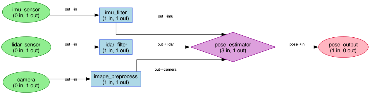
Robotics systems process data from multiple sensors simultaneously—cameras, IMUs, LiDAR. Each sensor feeds into processing nodes that transform, filter, and fuse data before outputting control signals. A compute graph models this as a directed acyclic graph where nodes are processing units and edges are data flows.
nodix executes these graphs with real-time guarantees. Nodes declare their deadlines and data dependencies. The scheduler (EDF or Rate Monotonic) ensures high-priority nodes meet their deadlines. If your camera runs at 30fps and your control loop needs 1000Hz, the scheduler handles it.
I tried my best to get this done in a single week and that turned out to be a herculean effort but I am glad I pushed to iterate this quickly. It was fun and I was able to push my limits and learn a lot.
Architecture
The system has four node types:
- Source: Produces data (sensors, timers)
- Filter: Transforms single inputs (detection, preprocessing)
- Fusion: Combines multiple inputs (sensor fusion, state estimation)
- Sink: Consumes data (actuators, logging)
Nodes connect through typed ports. A node declares input/output ports with specific data types. The graph validates connections at construction—you can’t wire an image port to an IMU port.
Two executors are available. The single-threaded executor processes nodes in topological order—deterministic but limited throughput. The parallel executor distributes ready nodes across threads—higher throughput but requires careful synchronization.
Key Design Decisions
Zero-copy data flow. Large data (images, point clouds) is wrapped in Arc. Nodes receive shared references rather than copies. A 1080p image passes through five nodes without a single memcpy.
Pluggable scheduling. EDF (Earliest Deadline First) prioritizes urgent work. Rate Monotonic assigns static priorities based on period. FIFO and priority-based options exist for simpler cases. The scheduler is a trait—swap implementations without changing node code.
HDR histograms for latency. Every node records execution time in a histogram. p50, p99, max latencies are available at runtime. When a deadline is missed, you know exactly which node and by how much.
Challenges & Lessons
Determinism vs throughput is the core tension. Single-threaded execution is predictable but leaves cores idle. Parallel execution is fast but introduces scheduling jitter. The solution was making this an explicit choice—users pick the executor that fits their constraints.
Type safety across dynamic connections was tricky. Nodes are trait objects (dynamic dispatch) but ports are generic (static types). The compromise: runtime type checking at connection time, zero-cost after construction.
Debugging deadline misses required good tooling. Chrome tracing export lets you visualize exactly when each node ran. Combined with histograms, you can identify bottlenecks quickly.
Performance
- 5K+ iterations/sec throughput
- <1ms p99 latency
- Zero-copy for images, point clouds, tensors
What I’d Do Differently
The executor abstraction could be cleaner. Right now switching executors requires some boilerplate. A builder pattern would help.
I’d add more built-in nodes. Currently users implement everything. A library of common operations (rate limiting, buffering, basic transforms) would reduce friction.
I wanted to get this done in a few days but that turned out to be a herculean effort. This is still in early iteration. I think another month or two of tweaking and iterating will help me improve it further.